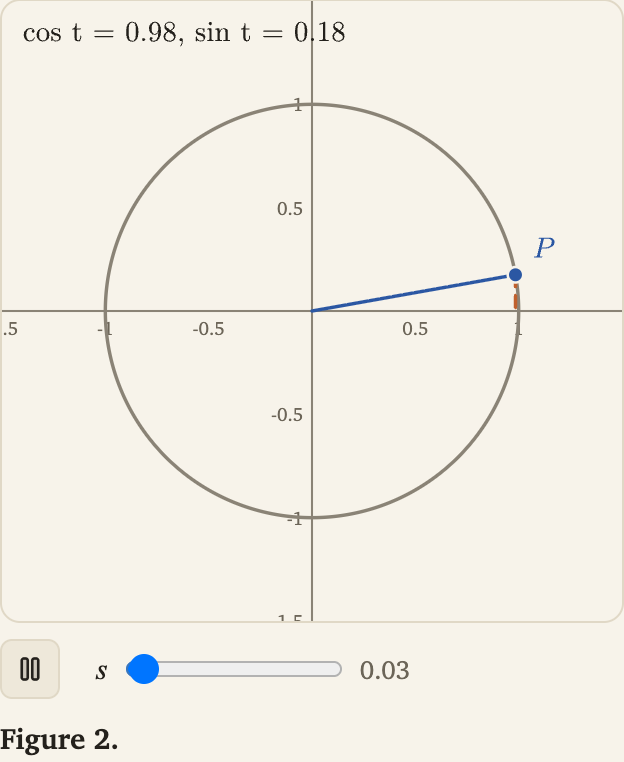
Figures
Room to Prove comes with a library of figures. You don't need to write anything to use them.
- Take one from the library. Open the Figure library. Filter by field, level and topic. Copy one into a lesson.
- Ask the assistant. Describe the figure, or the change you want. It writes it, checks it and fixes what the check finds.
- Keep your own. It goes in the library, next to the others.
Every number a figure shows is computed by the figure itself.
Adjusting a figure by hand
A figure is a few lines, one statement per line:
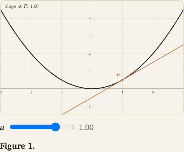
```figure
view x -3..3, y -1.5..5 grid
f(x) = x^2 / 2
a = slider(1, -2, 2)
graph f thick
tangent(f, a) secondary
P = point(a, f(a)) secondary label="$P$" at=above_left
text(-2.9, 4.9, "slope at $P$: #{f'(a):2}") at=below_right
```
viewsets the window.f(x) = …defines a function.f'is its exact derivative.slidermakes a value the reader moves.#{…}shows a computed value in a caption.
Motion
param is a clock. animate 6s loop plays it.
What a figure can hold
| Kind | Examples |
|---|---|
| Marks | point, segment, circle, polygon, graph, tangent, area, curve, surface, tree, table, text and more |
| Moving parts | slider, param … animate, points you drag |
| Algorithms | mergesort(…), rectree(…), mlp(…), walked step by step |
| Space | a 3D view with a camera; curves and surfaces |
| Colours | the theme's: accent, secondary, green, red, purple, orange, muted |
For agents
The assistant has five figure tools:
figure_scenarios: find a figure in the library, or one of yours.figure_from_scenario: build it.figure_check: check it, and describe what it draws.figure_edit: change it.figure_reference: the complete reference below.
The complete reference
Made from the app itself:
One statement per line; # starts a comment. Names must be defined above where they are used. Angles are in radians.
Statements
view x a..b, y c..d [grid] [noaxes] [size WxH] [xlabel="…"] [ylabel="…"]view x a..b, y c..d, z e..f [camera(az, el)] [perspective] [zoom k] [box] [grid] [noaxes] [size WxH]: a view in space. The camera turns by azimuth about z and elevation above the xy-plane, in radians, as expressions (a slider or the clock may turn it); the reader turns it by dragging. Shapes are drawn far to near and lit; every mark takes points in space (z is 0 where a point has none);text(x, y, …)is a caption placed on the screen by the x and y ranges,label(P, …)sits at Pf(x) = expr: a function;f'(x)is its exact derivativea = slider(value, min, max[, step]);t = param(from, to) animate 4s loop|bounce|once: the clock for animationsname = expr: a value; a point value is drawn unlesshidden- a mark (below), with styles after it and
when exprto draw it only while expr is non-zero T = producer(…): a dataset computed by the app;s = step(T)walks its steps. Producers:- mergesort: mergesort(5, 2, 4, 7, …): every split, comparison and copy of a top-down merge sort, splitting as Lean's List.mergeSort does
- insertionsort: insertionsort(5, 2, 4, …): each comparison and shift of insertion sort
- binarysearch: binarysearch(target, 1, 3, 4, …): binary search for target in the sorted numbers that follow
- mergetree: mergetree(5, 2, 4, 7, …): the call tree of merge sort, splits top-down, then merges bottom-up
- rectree: rectree(a, b, n, c=1, symbolic=0): the recursion tree of T(n) = a T(n/b) + n^c, with the cost of each level
- comparisons: comparisons(maxN): comparisons merge sort makes, worst case and on random input, beside n log2 n
- cayley: cayley(n, op="add", sub=k): the operation table of ℤ/nℤ under + (or of its units under ·, op="mul"); with sub=k, one step per coset of the subgroup ⟨k⟩
- mlp: mlp(2, 8, 8, 1, epochs=…, lr=…, seed=…, activation="tanh"): a network trained by gradient descent on two moons, snapshots of every stage
- phaseplot: phaseplot("(z - 1) / (z^2 + 1)", x0, x1, y0, y1, cols, rows, bands=5): arg f(z) in equal sectors, a domain-colouring picture of a complex function
- mandelbrot: mandelbrot(x0, x1, y0, y1, cols, rows, maxit=200, frames=12): escape times of z ↦ z² + c from z = 0, c on the grid; frames allow more iterations
- julia: julia(cx, cy, x0, x1, y0, y1, cols, rows, maxit=200, frames=12): escape times of z ↦ z² + c from each z on the grid (the filled Julia set of c)
- newton: newton("z^3 - 1", x0, x1, y0, y1, cols, rows, steps=30): Newton's method from every point of the grid, one frame per step, coloured by the root reached (basins of attraction)
- bifurcation: bifurcation("r * x * (1 - x)", r0, r1, x0, x1, cols, rows, warm=400, keep=300, start=0.5): where the orbit of x ↦ g(x, r) settles, for each r (a bifurcation diagram)
- markov: markov("0.9 0.1; 0.5 0.5", start=0, steps=20): a Markov chain's distribution π_t = π_0 Pᵗ step by step, beside its limit, with the distance ½Σ|π_t − π| (rows separated by ";")
- ulam: ulam(size, start=1, mark="none", note=0): the Ulam spiral of side size (odd, at most 401) from start, primes shaded; mark="euler" or "twin" picks out n² + n + 41 or twin primes; note=1 writes the count of primes
- heapops: heapops(5, 3, 8, …, kind="min"|"max", build="insert"|"heapify", extracts=2): a binary heap built, then its root extracted, every comparison and swap
- bst: bst(5, 3, 8, …, delete="3 8"): keys inserted into a binary search tree in that order, then deleted; the keys and each step
- unionfind: unionfind(n, "0-1, 2-3, ?3", rank=1, compression="full"|"halving"|"none"): a disjoint-set forest, its parent array step by step
- calltree: calltree("fibonacci"|"binomial"|"hanoi"|"fast_power", n, k=0, memo=0, counts=1): the tree of recursive calls, each value as it returns
- graphrun: graphrun("bfs"|"dfs"|"dijkstra"|"bellman_ford"|"prim"|"kruskal"|"topological", "A-B:4, B-C:2" or a preset, source="A"): a graph algorithm step by step, its arrays and notes
- dfarun: dfarun("A 0 B; A 1 A; B 0 B; B 1 A", "B", "0110", mod=0): a DFA reading its input; with mod=k its states are remainders of a binary number
- subset: subset("0 a 0; 0 b 0; 0 a 1; 1 b 2", "2"): the subset construction of a DFA from an NFA (eps for ε-moves), its table step by step
- turing: turing("increment"|"unary_add"|"palindrome"|"busy_beaver_2"|"busy_beaver_3"|"busy_beaver_4", input): a Turing machine's tape, head and state, step by step
- modexp: modexp(b, e, m, method="ltr"|"rtl"): b^e mod m by square-and-multiply, bit by bit
- descent: descent("x^2 + 10 y^2", x0, y0, method="gd"|"momentum"|"nesterov"|"rmsprop"|"adam", lr=0.05, steps=100, beta=0.9): an optimiser's path on f(x, y), with the exact gradient
- kmeans: kmeans(k, n=200, seed=1, data="blobs"|"uneven"|"elongated"|"rings"|"moons"|"uniform", spread=0.5, init="random"|"plusplus"): Lloyd's iterations, each assignment and update
- knn: knn(n=120, noise=0.2, seed=1, data="moons"|"circles"|"xor"|"blobs"|"spiral", metric="euclidean"|"manhattan"|"chebyshev"): the k-nearest-neighbour vote over the plane, one step per k = 1, 3, 5, …
- linclass: linclass(n=60, gap=2.5, spread=0.8, seed=1, method="perceptron"|"logistic", lr=1, epochs=50): a linear classifier learning, its boundary over the plane
- selectionsort: selectionsort(5, 2, 4, …): each comparison and swap of selection sort
- bubblesort: bubblesort(5, 2, 4, …): each comparison and swap of bubble sort, stopping early after a pass with no swap
- quicksort_lomuto: quicksort_lomuto(5, 2, 4, …): quicksort with the Lomuto partition (the last element as pivot)
- quicksort_hoare: quicksort_hoare(5, 2, 4, …): quicksort with the Hoare partition (the middle element as pivot)
- heapsort: heapsort(5, 2, 4, …): heapsort in place: build a max-heap, then move the root to the end, again and again
- shellsort: shellsort(5, 2, 4, …, gaps="shell"|"knuth"|"ciura"): Shell's sort, insertion sort on items a gap apart for shrinking gaps
- countingsort: countingsort(5, 2, 4, …): counting sort of whole numbers from 0 to 20: count, sum, place
- dptable: dptable("lcs"|"edit", "ABCBDAB", "BDCABA") or dptable("knapsack", "1 3 4 5", "1 4 5 7", capacity=7) or dptable("coins", "1 3 4", "", amount=6): a dynamic-programming table filled cell by cell, then traced back
- strmatch: strmatch("naive"|"kmp"|"rabin_karp", "text", "pattern", q=13): every comparison of a string search; KMP builds its failure table first
- hashtable: hashtable("chaining"|"linear"|"quadratic"|"double", m, key, key, …): keys inserted one by one into m slots with h(k) = k mod m, every probe and collision
- orbital: orbital(n, l, m, R): the probability density |ψ_nlm|² of a hydrogen orbital (real form) on the plane through the z axis where its lobes lie, over [−R, R]², shaded on a square-root scale
Values
Numbers, points (in the plane, or in space with point(x, y, z)) and lists. Operators + - * / ^, comparisons, && ||; A.x, A.y, A.z; xs[i] (from 0); [a, b, c]; [f(k) for k in range(n)]. Constants: pi, e, tau. A function may return a point: c(t) = point(cos(t), sin(t), t/4) is a curve, r(u, v) = point(…) a surface, and c'(t) its exact derivative.
- numbers: sin, cos, tan, asin, acos, atan, atan2, sinh, cosh, tanh, exp, ln, log, log2, sqrt, cbrt, abs, sign, floor, ceil, round, min, max, sigmoid, relu, clamp, gamma, lgamma, erf, binom
- geometry: point, midpoint, dist, slope, centroid, circumcenter, circumradius, incenter, inradius, orthocenter, foot, reflect, rotate, polar, angle, deg
- calculus: root, integral, lsum, rsum, msum, taylor (their first argument is an expression in x)
- len(xs): how many elements xs has
- range(n), range(a, b), range(a, b, step): the numbers from a (0) up to but not including b
- sum(xs): the sum of numbers or of points
- prod(xs): the product of numbers (1 for none)
- cumsum(xs): the running sums [x0, x0 + x1, …], of numbers or points
- lerp(a, b, u): from a (u = 0) to b (u = 1), for numbers or points
- cond(c, a, b): a if c is non-zero, else b; only the chosen one is evaluated
- mod(a, b): the remainder of a by b, never negative for b > 0
- phase(t, a, b): 0 before a, 1 after b, rising linearly between (timing)
- ease(u): u eased in and out (cubic), for u in [0, 1]
- ease_in(u): starts slowly (cubic)
- ease_out(u): ends slowly (cubic)
- smooth(u): smoothstep, 3u² − 2u³
- rand(i), rand(i, seed): a fixed "random" number in [0, 1) for each whole number i; the same every time
- dot(a, b): the dot product of two vectors (points), in the plane or in space
- cross(a, b): the cross product, a vector in space (z is 0 where a point has none)
- norm(a): the length of a vector
- unit(a): a / norm(a), the vector of length 1 along a
- curves and surfaces, by the name of their function, from its exact derivatives:
- partial(r, k, u, v, …): the derivative of r in its k-th parameter (from 1); partial(r, [1, 2], u, v) for r_uv
- speed(c, t): |c'(t)|
- curvature(c, t): κ, signed for a plane curve
- torsion(c, t): τ of a space curve (0 for a plane one)
- frenet_t(c, t): the unit tangent T
- frenet_n(c, t): the unit normal N (towards the centre of curvature)
- frenet_b(c, t): the binormal B = T × N
- arclength(c, a, b): the length of c from t = a to t = b
- normal(r, u, v): the unit normal r_u × r_v / |r_u × r_v|
- first_form(r, u, v): [E, F, G], the metric
- second_form(r, u, v): [L, M, N] against the unit normal
- gauss(r, u, v): the Gaussian curvature K = (LN − M²)/(EG − F²)
- mean_curvature(r, u, v): H = (EN − 2FM + GL)/(2(EG − F²))
- principal(r, u, v): [κ1, κ2], the principal curvatures, κ1 ≥ κ2
Marks
- P = point(x, y) [drag]: a point;
dragmoves the sliders it is made of - segment(A, B)
- line(A, B): the whole line through A and B
- ray(A, B): from A through B
- vector(A, B): an arrow from A to B
- circle(C, r) or circle(C, P): by radius or through P
- polygon(A, B, C, …): points or lists of points; closed
- graph f, or graph(f, from, to[, s…]): y = f(x) for a function f(x) = … defined above; for c(t) = point(…) the curve t ↦ c(t), in the plane or in space (n=400 samples). Further arguments go to the function after its first (a family, a homotopy)
- tangent(f, x0)
- area(f, a, b): the area under f
- label(P, "text with ")
- text(x, y, "text with and #{expr}")
- riemann(f, a, b, n, "left" | "right" | "mid")
- ngon(O, r, n, phase): a regular n-gon
- anglemark(A, B, C): the angle at B
- array(T, s[, x0, y0]): step s of a trace dataset
- tree(R[, s[, x0, y0, x1, y1]]): a tree dataset
- network(N, s, P, x0, y0, x1, y1[, t]): a trained network on the input P
- field(N, s): a network's output as a heat map
- contour(N, s, level)
- scatter(N): a dataset's points
- curve(S[, s]) or curve(N, s, x0, y0, x1, y1): a series, or a training run's loss
- table(T, s[, x0, y0]): a group table dataset
- rect(x, y, w, h): from the lower-left corner
- ellipse(C, rx, ry)
- arc(C, r, a0, a1): angles in radians
- wedge(C, r, a0, a1): a closed sector (pie charts)
- polyline(A, B, …): points or lists of points; open
- path("M 0 0 L 1 2 C 2 2 3 1 3 0 Z"): SVG commands M L H V C Q Z (lower case relative) in data coordinates; #{expr} puts in a number, or a point as two
- surface(r, u0, u1, v0, v1[, s…]): the surface r(u, v) = point(x, y, z) over a rectangle, lit; n=24 or n=48x12 faces, lines=8 or lines=12x6 parameter lines, flat, opacity=, where=(…) keeps a face and heat=(…) colours it by a number in [0, 1] through colors=a,b[,c], both with u, v and the face centre x, y, z bound. In a plane view, r(u, v) = point(x, y) draws a chart: the image of the parameter grid
- tube(c, a, b, radius[, s…]): a tube around the space curve c(t), t from a to b (knots, links); styles as for surface
- implicit(F[, c]): the level set F(x, y) = c in a plane view; n=160 cells across
- vectorfield(V[, n]): arrows of the field V(x, y) = point(…) on an n-wide grid (15), scaled to fit
- flowline(V, P, T[, steps]): the integral curve of V from P for time T (negative: backwards); V(x, y) in the plane, V(x, y, z) in space
- glue(A, B, k): the edge from A to B with k arrowheads at its middle, for gluing diagrams (a torus from a square)
Styles
- colours: accent, secondary, green, red, purple, orange, muted, ink, or
color=name/fill=namewith a CSS colour word or #rrggbb;fill=palette(i)cycles accent, secondary, green, purple, orange, red dashed,dotted,thick,thin,hidden,label="…", positions above, below, left, right (andat=below_leftetc.)width=,size=,opacity=anddraw=take a number or an expression in brackets:opacity=(1 - t).draw=(u)draws a line up to the fraction u of its length- a closed shape is filled only with
fill=…
Blocks
A header ending in :, and the lines indented under it. Names assigned inside a block are local to it.
def name(a, b):a component, called as a statementname(1, 2) [when …]; it sees its parameters and the names defined above it, and may call itselffor v in list:the body once per elementif cond:the body while cond is non-zerogroup translate(x, y) rotate(a[, P]) scale(s[, sy]):the body drawn through the transforms, applied right to left as in SVG; a point in a group cannot be dragged Sliders, datasets, functions anddefare only at the top level.
Timing
Make a clock t = param(0, 1) animate 4s once and compute from it: phase(t, a, b) for a stage, ease(u) to soften it, phase(t, i / n, i / n + 0.3) to stagger elements.
Limits per frame
20,000 shapes, 100,000 loop steps and calls, components nested 24 deep, lists of 100,000 from range. Passing one stops that statement with an error.
Examples
A bar chart that grows:
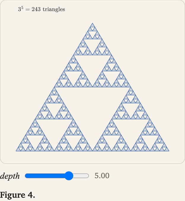
The Sierpiński triangle: